Welcome to Audio Over IP

In this inaugral blog post, we’ll explain the wonders of computerised audio, networked audio, and the magic that makes up a modern broadcast chain.

This guide is meant for people who have a good understanding of ‘traditional’ broadcast engineering and who want to extend that into the digital and IP domains!

Pulse Code Modulation (or ‘PCM’) – or audio sampling – is the cornerstone of all digital audio.

The concept is relatively simple: you take a sample (measure the volume) of an analogue signal 𝑛 times per second. If you later re-produce this, you can re-create the original signal with pretty good accuracy.

How many times per second do we sample the signal?

The rule of thumb is you need to take 2 x the maximum frequency you want to record (called the ‘Nyquist’ frequency). Given humans generally can’t hear above 20 kHz, we sample above ~40 kHz, or around 40,000 times a second. Two popular sampling rates are 44.1 kHz and 48 kHz.

Harmonic Distortion When Sampling

But what happens to the audio frequencies above ½ the sample rate? If we don’t do anything - these create harmonic distortions (aliasing) in our signal.

To fix that, there are two techniques that are used during Analogue to Digital conversion.

The first is to use a low-pass filter, to prevent frequencies above our Nyquist frequency from being sampled.

As most engineers will know, low-pass filter isn’t perfect, so to compensate, the higher-end sound cards will use a higher sampling rate (typically double again) – and then ‘down convert’.

Time vs Frequency Domain

Time-domain simply refers to measurements taken over time. In its simplest form, this just means recording a sequence of each sample. A WAV file is an example of a time-domain format for storing audio. 

Like from going from 2D to 3D, you can compute a signal between the time domain and the frequency domain. This is the precursor to most digital signal processing.

The frequency domain is a slice-in-time of what frequencies were present.

Now we’ve captured our audio samples, we might want to store or transmit them in a lossy format, such as MP3 or AAC.

We could also use a lossless format like WAV or FLAC, or even using a technique called an Adaptive Pulse Code Modulation (ADPCM).

But what does this mean and how do these work?

Lossless codecs – like the name suggest – give perfect reconstruction of the audio signal. This will inherently take up more storage space, as we have to fit 48,000 samples * duration into a file.

Lossy codecs were born when the internet needed a way of sending audio over dial-up – or, prior to that, public telephone networks.

There are two different types of lossy codecs – time-domain and frequency-domain.

Time-domain codecs, such as Adaptive Differential PCM, are relatively simple. They work by reducing the dynamic range, meaning less bytes are needed to store each sample. It’s not too dissimilar to compression in analogue audio.

Frequency-domain codecs (MP3, AAC), as the name suggests, will transform the audio into the frequency domain first. They then work by, in effect, making a table of frequencies, and an envelope of their loudness (what time they start, and what time they end, and the volumes between).

But how do we convert our sound wave into the frequency domain? The answer is with a complicated mathematical function called the Fourier transform. Specifically, we use the Discrete Time Fourier transform (DTFT).

This is a lot more efficient to store, but, because Discrete Time Fourier transforms aren’t perfect, it will never give a perfect recreation of the original signal. This is because the DFT, being a discrete mathematical function, only has the resolution of N different frequencies – where N reduces as you work with less audio – so most frequencies get rounded up or down to fit into one of those frequency ‘bins’.

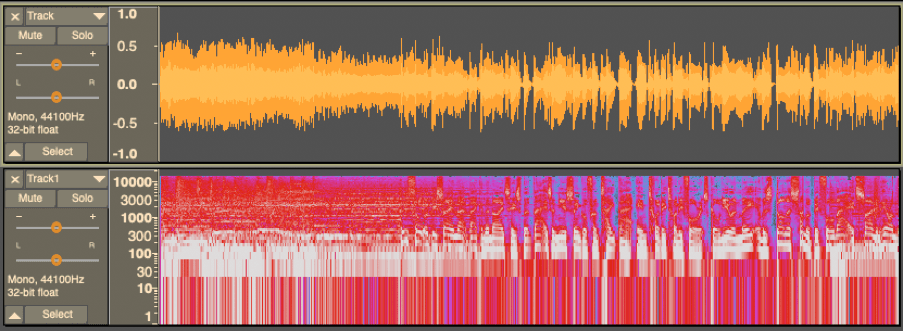
So, it's a trade off - do you want more time resolution, or more frequency resolution?

Let's have a look at that on a spectograph.

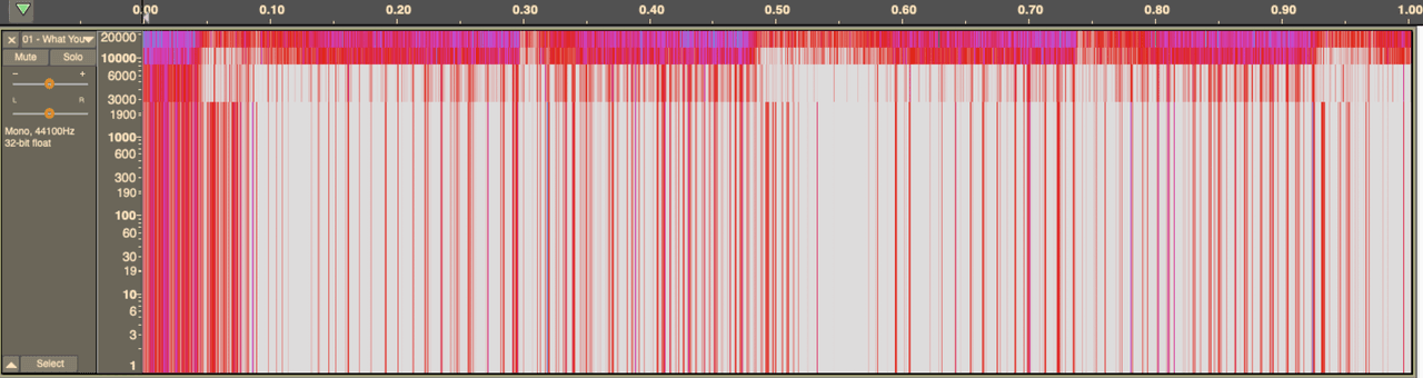
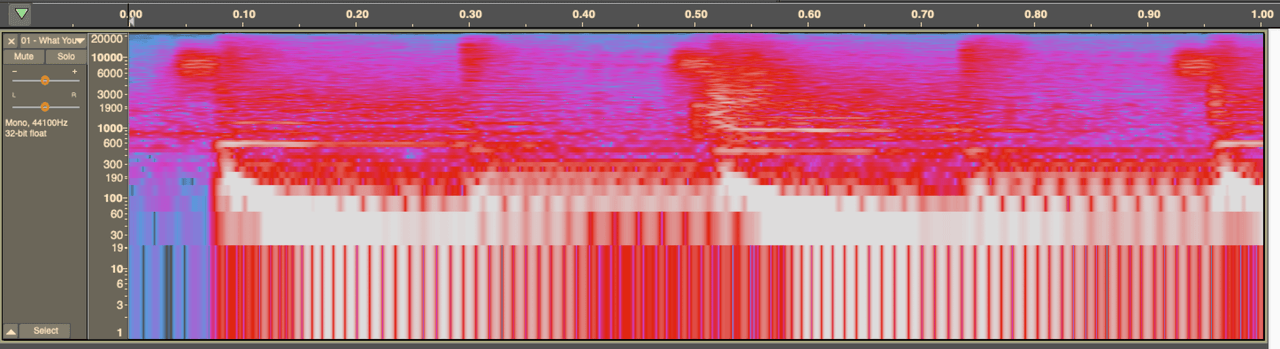
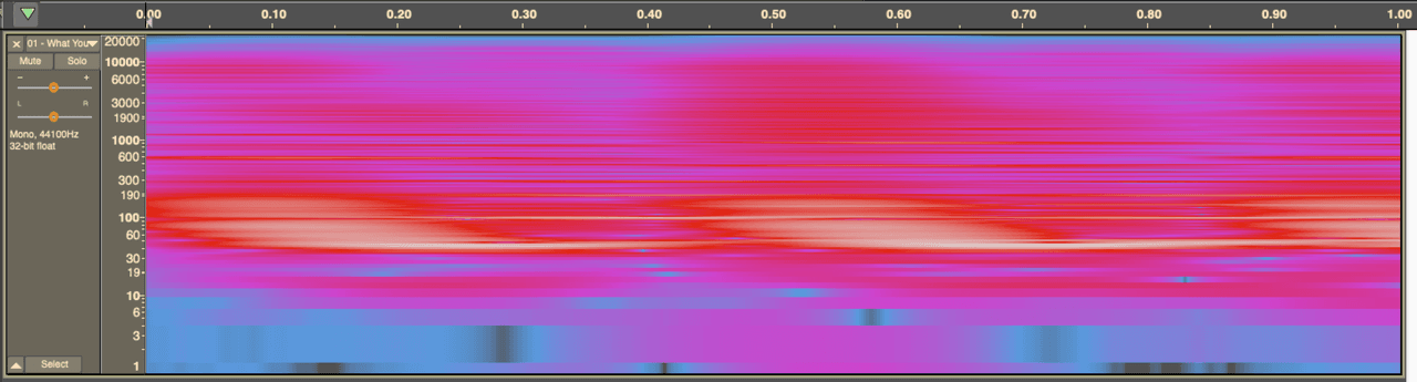
When you lower the bit rate, these codecs will ‘drop’ the quietest frequencies, or use ‘psycho-acoustic’ models to drop frequencies a human won’t find as important. This saves on storage space, but is very noticeable to the ear.

The biggest issue with frequency-domain codecs is that each round of coding loses important information, further reducing the quality.

In an ideal world, lossy codecs should only ever be used for distribution to the end-listener, and never as a production format! If only it was that easy...

This is very similar to saving a JPEG photo multiple times and noticing the graininess increase.

As we know, unlike analogue audio, digital audio has delay/latency.

But hold on… If we’re sampling the audio 48,000 times a second, why is that delay any higher than 1/48000^th of a second?

This comes down to the fact that audio processing works in chunks (buffers) of, say, 1000 samples (about 20ms) at a time. Some algorithms, like the Fourier transform, need quite a few samples to work on, otherwise the frequency resolution is not very good.

But more simply – doing an action on a computer 48,000 times a second is very intensive.

Even though modern processors compute billions of instructions a second, it’s magnitudes more efficient to process a 20ms section of audio 48 times a second, than 0.02ms of audio 48,000 times a second. This is because inside any modern operating system, it takes (relatively) a lot of work to switch between tasks (e.g. other programs).

For the same reason, a sound card will only pass sound to/from the computer e.g. 48 times a second.

As we’ve explored, we can only work on one buffer at a time. That means, from analogue to end-application (e.g. Audacity), the delay will be about 3 buffers – 1 buffer inside the sound card, (at least) 1 inside the operating system, and 1 inside the application.

Technologies like ASIO tried to reduce this delay by giving an application direct access to the buffer on the sound card. Complex processing chains (think Stereo Tool) might create a "pipeline" to apply multiple steps to a single buffer.

On a busy computer, one buffer might not be long enough. The computer will form a “queue” of buffers.

Imagine a bucket of water with some holes in the side, but near the bottom.

If we fill it faster than it drains, the water level goes up – this is our buffer.

If we don’t fill the bucket fast enough, water will stop flowing. We call this a buffer underrun (or underflow). And we don’t want to fill the bucket too high or it will overrun/overflow.

Longer buffers, are generally associated with better reliability, with the trade-off of latency.

Long buffers are particularly important over the public internet, where the end-to-end delay might be 1ms 90% of the time, but 10ms 9% of the time, and 100ms 1% of the time. The system designer needs to decide whether to accept the 100ms delay, or to aim less, and accept the occasional drop-out where the bucket becomes empty (e.g. VOIP calls).

You might have noticed a “SYNC” XLR socket on the back of your AES/EBU equipment, and wondered why you might ever need to use it.

Welcome to one of the biggest headaches in digital audio.

Hark back to our foundation stone of audio sampling. If we’re sampling an audio signal 48,000 times a second, how does the ADC know what a second is?

Inside a closed system – where there is one clock – the answer is fairly straightforward – everything uses this clock as its source of truth.

But this model quickly collapses when you begin to combine different systems with different clocks. Often you won’t have a choice in this – for example, if you want to connect an AES67 stream to a USB sound card (which has its own built-in clock). Although it might work… kind of… the audio will probably be very choppy. But why?

Short of atomic ones, computer clocks aren’t perfect. They generally rely on the oscillation of a crystal, and – as you may know from demodulating FM – will gradually slow down over time.

If you end up with a clock running at 48,000.001 Hz and another at 47,999.999 Hz, although they will mostly be in sync, after a few minutes they will not be.

Consider the leaky bucket model - what would happen if the source is running at a slightly slower rate than the sink?

Professional implementations of Dante/Livewire/AES67/etc. generally solve this problem by avoiding having multiple clocks. In an AES67 compatible system, one device is usually [automatically] elected to be the “master” clock, and everything else will run off this time.

This works using a feature of modern computer networks called Precision Time Protocol (version 2) – which is designed to distribute a highly accurate time-code.

PTPv2 is recognised and prioritised in a modern network switch – although it will work on older switches, there is no “quality of service” guarantee, so it may not perform as well.

A software/virtual sound card, unlike a USB sound card – which is clocked by a crystal on the device itself – is generating its clock from the PTPv2 signal. Similarly, an ‘edge’ device, like an Axia XNode, does its sampling based on this signal.

How does this work? An algorithm based on a Phase or Delay Locked Loop creates a clock that is constantly synchronised according to the grandmaster time

Of course, avoiding the problem doesn’t solve the problem of bridging systems with different clock “boundaries” – for example, if you wanted to play a live stream from the internet through a virtual sound card.

Most free/consumer software, sadly, has no, or very naïve (e.g. audible through a pitch change), clock correction. This makes perfect streaming very difficult to achieve, as, over time – depending on how ‘skewed’ the clocks are – the delay will either grow, as the buffer gets bigger, or will pause and glitch, as the buffer underruns.

There are solutions to this, but they are complex (see Asynchronous Sample Rate Conversion) and the take-up by open source projects has been slow.

For example, ASRC used Barix Exstreamer that makes it much better at playing an Icecast/Shoutcast stream than VLC on a small form factor PC.

You may have heard of the Real Time Protocol or RTP – the network protocol that gets used to transmit low-latency audio (or video, etc)

RTP is, under the hood, an incredibly simple system. It sends a few buffers of audio, with an incrementing number - the sequence number. It’s been used for decades – most notably for Voice Over IP phone calls.

Generally, it is used in a Point to Point (or "unicast") fashion - one sending IP address transmits to a receiving IP address, on a specific port number.

RTP is just the audio data stream – coordinating the start/end of a RTP stream, any extra parameters or extensions, metadata etc., happens elsewhere.

In most systems, a variant of “Session Description Protocol” is used, in conjunction with (usually a proprietery) discovery mechanism.

RTP generally works on a “unicast” or point-to-point basis (one sending device is sending to one receiving device).

But what if we want to send one audio stream to multiple destinations inside our Local Area Network?

For this, we use a multicast system.

On your LAN, you probably use IP addresses starting 192.168 or 10. These are known as internally reserved IP addresses. There are some separate IP addresses reserved for multicast - they are: 224.0.0.0 - 239.255.255.255

(Note that multicast only exists inside a LAN - it's not possible to transmit a multicast flow over the public internet)

A multicast sender creates a group by choosing a free IP address. It then advertises this through some mechanism (such as the Session Description Protocol over 'mDNS')

A listener can ask to join (or leave) the multicast group. The network switch will then start sending the listening device all the new audio buffers.

Icecast (or Shoutcast) streaming servers work based on unicast model, but they do effectively simulate the multicast experience.